Introduction to SportsLabKit#
This quick tutorial introduces the key concepts and basic features of SportsLabKit to help you get started with your projects.
Multiple Object Tracking in SportsLabKit#
In a broad definition, Multiple Object Tracking (MOT) is the problem of automatically identifying multiple objects in a video and representing them as a set of trajectories.
The typical approach to MOT algorithms follows the tracking-by-detection paradigm, which attempts to solve the problem by first detecting objects in each frame and then associating them with the objects in the previous frame.
One large challenge in the tracking-by-detection paradigm is scalability. The detection model is typically a deep learning model, which is computationally expensive. The association model is also computationally expensive, as it requires reID features to be extracted for each bounding box. Recent approaches, such as TrackFormer/TransTrack, have attempted to address this challenge by using a single deep learning model to perform both detection and association. However, there is no clear consensus on the best approach to MOT as tracking-by-detection models are still competitive (ByteTrack/BoT-SORT/Strong-SORT).
IMHO, approaches that adhere to “The Bitter Lesson” are the most promising. Unicorn: Towards Grand Unification of Object Tracking demonstrates that a single network can solve four tracking problems (SOT, MOT, VOS, MOTS) simultaneously. I think this is a direction many will follow.
SportsLabKit implements the tracking-by-detection paradigm.
In brief, the algorithm works as follows:
The detection model (YOLOX, DETR, RCNN etc.) detects items of interest via bounding boxes in each frame, then
Several feature extractors are used to obtain descripters of each detection (e.g. ReID features, optical flow features, etc.), then
The association model (Minimum cost bipartite matching) associates detections in the current frame with detections in the previous frame / existing tracklets.
For a more detailed explanation of the tracking-by-detection paradigm, please refer to the original DeepSORT paper, this blog explaining DeepSORT or our SoccerTrack paper.
![]()
We chose to start with this approach for two reasons: 1) it is a simple and modular approach and 2) we can explicitly control the use of appearance and motion features.
DataFrames in SportsLabKit#
SportsLabKit extends the popular data science library pandas by adding an interface to handle tracking data. If you are not familiar with pandas, we recommend taking a quick look at its Getting started documentation before proceeding.
There are two core data structures in SportsLabKit, the BoundingBoxDataFrame and the CoordinateDataFrame. Both are,
Subclasses of pandas.DataFrame and inherit all of its functionality
Inherited from the
SLKMixinand are designed to work with theSportsLabKitAPI
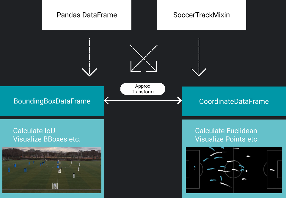
The main difference is that the CoordinateDataFrame has comes built-in with functionality that handles coordinates, while the BoundingBoxDataFrame is made to be compatibile with bounding box data.
In a nutshell, both data structures are a multi-indexed pandas.DataFrame with a few extra methods and attributes/metadata. This means that we can use various dataframe method directly:
df.head()returns the first 5 rows of the dataframedf.columnsreturns the column namesdf.iloc[0]returns the first row of the dataframe
While also extending functionality to additional convenience functions like:
df.iter_frames()iterates over the data frame by framedf.iter_teams()iterates over the data frame by teamdf.iter_players()iterates over the data frame by playerdf.iter_attributes()iterates over the data frame by attribute
See more about how to use dataframes in the DataFrame Manipulation tutorial.
Reading and writing files#
First, we need to read some data.
Reading files#
Assuming you have a file containing either bounding box or coordinates data, you can read it using slk.read_data(), which automatically detects the filetype and creates a BBoxDataFrame or a CoordinateDataFrame. This tutorial uses a sample from the SoccerTrack dataset, which is part of the SoccerTrack installation. Therefore, we use slk.datasets.get_path() to retrieve the path to the dataset.
%load_ext autoreload
%autoreload 2
import sportslabkit as slk
from sportslabkit.logger import show_df # This just makes the df viewable in the notebook.


dataset_path = slk.datasets.get_path("wide_view")
path_to_csv = sorted(dataset_path.glob("annotations/*.csv"))[0]

bbdf = slk.load_df(path_to_csv)

bbdf.head()
| TeamID | 0 | ... | 1 | 3 | |||||||||||||||||
|---|---|---|---|---|---|---|---|---|---|---|---|---|---|---|---|---|---|---|---|---|---|
| PlayerID | 1 | 10 | ... | 9 | 0 | ||||||||||||||||
| Attributes | bb_left | bb_top | bb_width | bb_height | conf | bb_left | bb_top | bb_width | bb_height | conf | ... | bb_left | bb_top | bb_width | bb_height | conf | bb_left | bb_top | bb_width | bb_height | conf |
| frame | |||||||||||||||||||||
| 0 | 3543.0 | 607.0 | 30.0 | 52.5 | 1.0 | 3536.42 | 555.93 | 13.57 | 42.39 | 1.0 | ... | 2919.31 | 538.44 | 23.59 | 47.18 | 1.0 | 3542.77 | 549.47 | 6.4 | 7.0 | 1.0 |
| 1 | 3542.0 | 609.0 | 32.0 | 51.0 | 1.0 | 3536.13 | 555.96 | 13.66 | 42.27 | 1.0 | ... | 2919.44 | 538.55 | 23.59 | 47.18 | 1.0 | 3548.55 | 549.43 | 6.4 | 7.0 | 1.0 |
| 2 | 3542.0 | 611.0 | 32.0 | 50.0 | 1.0 | 3535.85 | 555.99 | 13.73 | 42.16 | 1.0 | ... | 2919.57 | 538.66 | 23.59 | 47.18 | 1.0 | 3554.32 | 549.40 | 6.4 | 7.0 | 1.0 |
| 3 | 3542.0 | 613.0 | 32.0 | 49.0 | 1.0 | 3535.57 | 556.02 | 13.80 | 42.04 | 1.0 | ... | 2919.70 | 538.77 | 23.59 | 47.18 | 1.0 | 3560.10 | 549.36 | 6.4 | 7.0 | 1.0 |
| 4 | 3539.0 | 615.0 | 36.0 | 46.0 | 1.0 | 3535.28 | 556.04 | 13.88 | 41.94 | 1.0 | ... | 2919.84 | 538.88 | 23.59 | 47.18 | 1.0 | 3565.87 | 549.33 | 6.4 | 7.0 | 1.0 |
5 rows × 115 columns
To use the full soccertrack dataset, see “Dataset Preparation”.
Writing files#
To write back to file use BBoxDataFrame.to_csv().
bbdf.to_csv("assets/soccertrack_sample.csv")
Visualization#
Now that we have a bounding box dataframe, we can visualize the results.
path_to_mp4 = sorted(dataset_path.glob("videos/*.mp4"))[0]
It is also possible to download full soccertrack dataset using soccertrack.datasets.Downloader. See “Dataset Preparation”. for more details.
The BBoxDataFrame has a built-in visualize_frame() method that can be used to visualize the bounding boxes in a single frame.
from sportslabkit.utils import cv2pil

frame_idx = 50
cam = slk.Camera(path_to_mp4)
frame = cam.get_frame(frame_idx)
resized_frame = cv2pil(bbdf.visualize_frame(frame_idx=frame_idx, frame=frame), False).resize((frame.shape[1]//8, frame.shape[0]//8))
The BBoxDataFrame also has a visualize_bbox() method built in. It returns generators containing a sequence of drawn bounding boxes, which can be passed to the make_video method of soccertrack.utils to output a video.
The following notebook will output bbox_FISH.mp4 in the current directory.
save_path = 'assets/visualize_frames.mp4'
bbdf_short = bbdf.iloc[:100].copy()
bbdf_short.visualize_frames(path_to_mp4, save_path)
Writing video: 100it [00:08, 11.88it/s]
Tracking#
Below we provide a snippiet of code that detects and tracks the players and ball in the downloaded video. First we define the components of our tracking pipeline.
Camera- A class that handles camera calibration and coordinate transformationsdetection_model: A detection model, such as YOLOX, DETR, etc.motion_model: A motion model that predicts the next position of the players and ball, such as Kalman Filter, Constant Velocity, etc.SORTTracker: A tracker based on the SORT algorithm.
Deciding how to architect the structure of the tracking part was very tricky and probably suboptimal. We are still working on improving this part of the library so there may be some breaking changes in the future.
from sportslabkit.utils import get_git_root
from sportslabkit.mot import SORTTracker

root = get_git_root()
cam = slk.Camera(path_to_mp4)

det_model = slk.detection_model.load('YOLOv8x', imgsz=640)
motion_model = slk.motion_model.load('KalmanFilter', dt=1/30, process_noise=10000, measurement_noise=10)

tracker = SORTTracker(detection_model=det_model, motion_model=motion_model)
tracker.track(cam[:100])
res = tracker.to_bbdf()
Tracking Progress:   0%|          | 0/100 [00:00<?, ?it/s][W NNPACK.cpp:64] Could not initialize NNPACK! Reason: Unsupported hardware.
Tracking Progress: 100%|██████████| 100/100 [03:47<00:00,  2.27s/it, Active: 1, Dead: 2]
save_path = "assets/tracking_results.mp4"
res.visualize_frames(cam.video_path, save_path)
Writing video: 97it [00:21, 4.47it/s]
What next?#
This tutorial is a work in progress. If you have any questions or suggestions, please feel free to reach out.