Dataframe Manipulation

A Quick Introduction to SportsLabKit’s DataFrames

SportsLabKit seamlessly extends the popular data science library pandas to handle sports tracking data effortlessly. If pandas is foreign territory for you, it’s a good idea to skim through its Getting Started guide first.

Core Data Structures

SportsLabKit introduces two power-packed DataFrames, built just for your sports analytics needs:

1. BoundingBoxDataFrame: Tailored to handle bounding box dimensions.

2. CoordinateDataFrame: Designed for coordinate-based tracking data.

Both these structures have two key features:

• They’re subclasses of pandas.DataFrame, so you can do everything you do with a standard DataFrame.

• They inherit from SLKMixin, which means they’re optimized to play well with the SportsLabKit API.

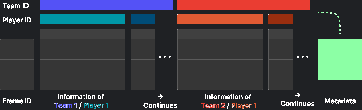
These are multi-level Pandas DataFrames with Team ID, Player ID, and other attributes. Each row is indexed by Frame ID.

Sample BoundingBoxDataFrame

import sportslabkit as slk

bbdf = slk.load_df('assets/sample_bbdf.csv')
bbdf.head()

TeamID	0										...	1					3
PlayerID	1					10					...	9					0
Attributes	bb_left	bb_top	bb_width	bb_height	conf	bb_left	bb_top	bb_width	bb_height	conf	...	bb_left	bb_top	bb_width	bb_height	conf	bb_left	bb_top	bb_width	bb_height	conf
frame
0	3543.0	607.0	30.0	52.5	1.0	3536.42	555.93	13.57	42.39	1.0	...	2919.31	538.44	23.59	47.18	1.0	3542.77	549.47	6.4	7.0	1.0
1	3542.0	609.0	32.0	51.0	1.0	3536.13	555.96	13.66	42.27	1.0	...	2919.44	538.55	23.59	47.18	1.0	3548.55	549.43	6.4	7.0	1.0
2	3542.0	611.0	32.0	50.0	1.0	3535.85	555.99	13.73	42.16	1.0	...	2919.57	538.66	23.59	47.18	1.0	3554.32	549.40	6.4	7.0	1.0
3	3542.0	613.0	32.0	49.0	1.0	3535.57	556.02	13.80	42.04	1.0	...	2919.70	538.77	23.59	47.18	1.0	3560.10	549.36	6.4	7.0	1.0
4	3539.0	615.0	36.0	46.0	1.0	3535.28	556.04	13.88	41.94	1.0	...	2919.84	538.88	23.59	47.18	1.0	3565.87	549.33	6.4	7.0	1.0

5 rows × 115 columns

Sample CoordinatesDataFrame

codf = slk.load_df('assets/sample_codf.csv')
codf.head()

TeamID	0										...	1							3
PlayerID	1			10			11			2	...	7	8			9			0
Attributes	x	y	conf	x	y	conf	x	y	conf	x	...	conf	x	y	conf	x	y	conf	x	y	conf
frame
0	53.133590	53.038124	1.0	52.62633	43.132626	1.0	54.01911	23.575058	1.0	68.94156	...	1.0	29.863533	52.299420	1.0	26.115326	41.902317	1.0	52.755344	31.830680	1.0
1	53.132770	53.099983	1.0	52.61572	43.114075	1.0	54.01330	23.639513	1.0	68.94156	...	1.0	29.885149	52.332210	1.0	26.135504	41.926130	1.0	53.072350	31.791082	1.0
2	53.131140	53.222996	1.0	52.60511	43.097652	1.0	54.00687	23.703869	1.0	68.76769	...	1.0	29.906412	52.364944	1.0	26.155657	41.949930	1.0	53.389380	31.754894	1.0
3	53.129520	53.345060	1.0	52.59448	43.079075	1.0	54.00056	23.763563	1.0	68.66287	...	1.0	29.927639	52.397614	1.0	26.175790	41.973686	1.0	53.707620	31.715126	1.0
4	53.098343	53.224068	1.0	52.58363	43.062626	1.0	53.99479	23.827623	1.0	68.76769	...	1.0	29.949121	52.430195	1.0	26.196299	41.997395	1.0	54.025840	31.678797	1.0

5 rows × 69 columns

Simple accessors and methods

Since the BBoxDataFrame and CoordinateDataFrame are subclasses of pandas.DataFrame, they inherit all of its functionality. This means that you can use all of the standard pandas.DataFrame methods and accessors.

For example,

• df.head() returns the first 5 rows of the dataframe

• df.columns returns the column names

• df.iloc[0] returns the first row of the dataframe

# bbdf.head() is used above!

print(bbdf.columns[0])

bbdf.iloc[[0]]

('0', '1', 'bb_left')

TeamID	0										...	1					3
PlayerID	1					10					...	9					0
Attributes	bb_left	bb_top	bb_width	bb_height	conf	bb_left	bb_top	bb_width	bb_height	conf	...	bb_left	bb_top	bb_width	bb_height	conf	bb_left	bb_top	bb_width	bb_height	conf
frame
0	3543.0	607.0	30.0	52.5	1.0	3536.42	555.93	13.57	42.39	1.0	...	2919.31	538.44	23.59	47.18	1.0	3542.77	549.47	6.4	7.0	1.0

1 rows × 115 columns

xs - Cross-section

Note that these are MultiIndex dataframes, so you can use more advanced indexing methods, such as df.xs.

In this example,

• df.xs(‘0’, level=’TeamID’, axis=1) returns the first team’s data

• df.xs(‘5’, level=’PlayerID’, axis=1) returns the data for player 5 in all teams

• df.xs((‘0’, ‘5’), level=(‘TeamID’, ‘PlayerID’), axis=1) returns the data for player 5 in team 0

bbdf.xs('0', level='TeamID', axis=1).head(3)

PlayerID	1					10					...	8					9
Attributes	bb_left	bb_top	bb_width	bb_height	conf	bb_left	bb_top	bb_width	bb_height	conf	...	bb_left	bb_top	bb_width	bb_height	conf	bb_left	bb_top	bb_width	bb_height	conf
frame
0	3543.0	607.0	30.0	52.5	1.0	3536.42	555.93	13.57	42.39	1.0	...	3457.05	803.91	72.0	88.0	1.0	3060.33	592.52	35.89	62.07	1.0
1	3542.0	609.0	32.0	51.0	1.0	3536.13	555.96	13.66	42.27	1.0	...	3455.43	802.76	72.0	88.0	1.0	3060.26	592.90	35.89	62.07	1.0
2	3542.0	611.0	32.0	50.0	1.0	3535.85	555.99	13.73	42.16	1.0	...	3450.35	801.80	72.0	88.0	1.0	3060.19	593.29	35.89	62.07	1.0

3 rows × 55 columns

bbdf.xs('5', level='PlayerID', axis=1).head(3)

TeamID	0					1
Attributes	bb_left	bb_top	bb_width	bb_height	conf	bb_left	bb_top	bb_width	bb_height	conf
frame
0	3720.0	504.0	12.0	27.0	1.0	3288.42	528.72	14.7	38.3	1.0
1	3720.0	504.0	12.0	27.0	1.0	3287.54	529.14	14.7	38.3	1.0
2	3720.0	504.0	12.0	27.0	1.0	3286.65	529.56	14.7	38.3	1.0

bbdf.xs(('0', '5'), level=('TeamID', 'PlayerID'), axis=1).head(3)

Attributes	bb_left	bb_top	bb_width	bb_height	conf
frame
0	3720.0	504.0	12.0	27.0	1.0
1	3720.0	504.0	12.0	27.0	1.0
2	3720.0	504.0	12.0	27.0	1.0

loc - MultiIndex slicing

MultiIndex slicing is a powerful tool for selecting data. Using the slice(None) object, you can select all data for a given index level. Although it’s a little verbose, it’s a very powerful tool once you get used to it.

In this example,

• df.loc[:, (‘0’, slice(None))] returns the data for team 0

• df.loc[:, (slice(None), ‘5’)] returns the data for team 0 player 5 in all teams

• df.loc[:, (slice(None), slice(None), ‘x’)] returns the x coordinates for all players in all teams

# Select all the columns from TeamID 0
bbdf.loc[:, '0'].head(3)

PlayerID	1					10					...	8					9
Attributes	bb_left	bb_top	bb_width	bb_height	conf	bb_left	bb_top	bb_width	bb_height	conf	...	bb_left	bb_top	bb_width	bb_height	conf	bb_left	bb_top	bb_width	bb_height	conf
frame
0	3543.0	607.0	30.0	52.5	1.0	3536.42	555.93	13.57	42.39	1.0	...	3457.05	803.91	72.0	88.0	1.0	3060.33	592.52	35.89	62.07	1.0
1	3542.0	609.0	32.0	51.0	1.0	3536.13	555.96	13.66	42.27	1.0	...	3455.43	802.76	72.0	88.0	1.0	3060.26	592.90	35.89	62.07	1.0
2	3542.0	611.0	32.0	50.0	1.0	3535.85	555.99	13.73	42.16	1.0	...	3450.35	801.80	72.0	88.0	1.0	3060.19	593.29	35.89	62.07	1.0

3 rows × 55 columns

# Select all the columns from TeamID 0 and PlayerID 5
bbdf.loc[:, ('0', '5')].head(3)

Attributes	bb_left	bb_top	bb_width	bb_height	conf
frame
0	3720.0	504.0	12.0	27.0	1.0
1	3720.0	504.0	12.0	27.0	1.0
2	3720.0	504.0	12.0	27.0	1.0

# Select all the columns containg `bb_left` in the name
bbdf.loc[:, (slice(None), slice(None), 'bb_left')].head(3)

TeamID	0										...	1									3
PlayerID	1	10	11	2	3	4	5	6	7	8	...	11	2	3	4	5	6	7	8	9	0
Attributes	bb_left	bb_left	bb_left	bb_left	bb_left	bb_left	bb_left	bb_left	bb_left	bb_left	...	bb_left	bb_left	bb_left	bb_left	bb_left	bb_left	bb_left	bb_left	bb_left	bb_left
frame
0	3543.0	3536.42	3560.51	3830.0	2671.0	4270.0	3720.0	3746.0	3818.0	3457.05	...	3184.08	3525.94	3529.66	3526.23	3288.42	3312.47	3336.58	2832.56	2919.31	3542.77
1	3542.0	3536.13	3560.44	3830.0	2671.0	4270.0	3720.0	3746.0	3818.0	3455.43	...	3184.20	3526.40	3531.11	3525.67	3287.54	3312.52	3336.72	2832.52	2919.44	3548.55
2	3542.0	3535.85	3560.36	3827.0	2670.5	4270.0	3720.0	3745.0	3818.0	3450.35	...	3184.33	3526.86	3532.57	3525.11	3286.65	3312.57	3336.86	2832.47	2919.57	3554.32

3 rows × 23 columns

Iterators

Both BBoxDataFrame and CoordinateDataFrame have several iterators that allow you to iterate over the data in different ways.

• df.iter_frames() iterates over the data frame by frame

• df.iter_teams() iterates over the data frame by team

• df.iter_players() iterates over the data frame by player

• df.iter_attributes() iterates over the data frame by attribute

See the API documentation for more details.

for player_idx, player_df in bbdf.iter_players(drop=False):
    print(player_idx)
    break

player_df.head(3)

('0', '1')

TeamID	0
PlayerID	1
Attributes	bb_left	bb_top	bb_width	bb_height	conf
frame
0	3543.0	607.0	30.0	52.5	1.0
1	3542.0	609.0	32.0	51.0	1.0
2	3542.0	611.0	32.0	50.0	1.0

Convert bbdf to codf

This is a quick guide to converting BoundingBox loaded on SoccerTrack to the pitch coordinate.

1. Load video and BoundingBox

import sportslabkit as slk
from sportslabkit.logger import show_df

dataset_path = slk.datasets.get_path("wide_view")
path_to_csv = sorted(dataset_path.glob("annotations/*.csv"))[0]
path_to_mp4 = sorted(dataset_path.glob("videos/*.mp4"))[0]

cam = slk.Camera(path_to_mp4)  # Camera object will be used to load frames
bbdf = slk.load_df(path_to_csv)  # We will use this as ground truth
bbdf.head()

TeamID	0										...	1					3
PlayerID	1					10					...	9					0
Attributes	bb_left	bb_top	bb_width	bb_height	conf	bb_left	bb_top	bb_width	bb_height	conf	...	bb_left	bb_top	bb_width	bb_height	conf	bb_left	bb_top	bb_width	bb_height	conf
frame
0	3543.0	607.0	30.0	52.5	1.0	3536.42	555.93	13.57	42.39	1.0	...	2919.31	538.44	23.59	47.18	1.0	3542.77	549.47	6.4	7.0	1.0
1	3542.0	609.0	32.0	51.0	1.0	3536.13	555.96	13.66	42.27	1.0	...	2919.44	538.55	23.59	47.18	1.0	3548.55	549.43	6.4	7.0	1.0
2	3542.0	611.0	32.0	50.0	1.0	3535.85	555.99	13.73	42.16	1.0	...	2919.57	538.66	23.59	47.18	1.0	3554.32	549.40	6.4	7.0	1.0
3	3542.0	613.0	32.0	49.0	1.0	3535.57	556.02	13.80	42.04	1.0	...	2919.70	538.77	23.59	47.18	1.0	3560.10	549.36	6.4	7.0	1.0
4	3539.0	615.0	36.0	46.0	1.0	3535.28	556.04	13.88	41.94	1.0	...	2919.84	538.88	23.59	47.18	1.0	3565.87	549.33	6.4	7.0	1.0

5 rows × 115 columns

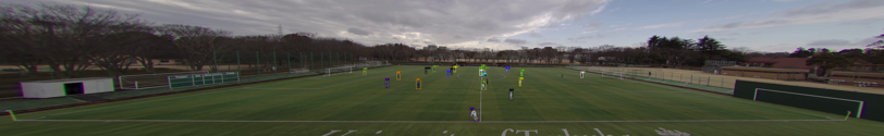
Now let’s visualize the loaded frames

frame = cam.get_frame(1)
vis_frame = bbdf.visualize_frame(1, frame)

slk.utils.cv2pil(vis_frame, convert_bgr2rgb=False).resize((vis_frame.shape[1] // 8, vis_frame.shape[0] // 8))

2. Convert BoundingBox coordinates to pitch coordinates

First, load the match video and the corresponding pitch keypoints, and then compute the projection matrix.

import numpy as np
from ast import literal_eval
import json 
from sportslabkit.utils import get_git_root, load_keypoints


keypoint_json = get_git_root() / 'notebooks/02_user_guide/assets/soccer_keypoints.json'
cam.source_keypoints, cam.target_keypoints = load_keypoints(keypoint_json)
print(cam.H)

[[  -0.022512    -0.15867      143.47]
 [  0.0039563    -0.25595      113.53]
 [ 5.8605e-05  -0.0030103           1]]

Based on the calculated projection matrix, the Bounding Box is projected onto the pitch coordinate.

The method argument can be used to the point within the bounding box to transform.
Options include center, bottom_middle, top_middle.

codf = bbdf.to_codf(cam.H, method='bottom_middle')
codf.head()

TeamID	0										...	1								3
PlayerID	1		10		11		2		3		...	6		7		8		9		0
Attributes	x	y	x	y	x	y	x	y	x	y	...	x	y	x	y	x	y	x	y	x	y
frame
0	53.133591	53.038124	52.626331	43.132626	54.019112	23.575058	68.941559	31.393507	8.064067	33.066338	...	40.216267	30.466066	39.744530	21.744230	29.863533	52.299419	26.115326	41.902317	52.755344	31.830681
1	53.132771	53.099983	52.615719	43.114075	54.013302	23.639513	68.941559	31.393507	8.064067	33.066338	...	40.227959	30.505083	39.757240	21.762505	29.885149	52.332211	26.135504	41.926128	53.072350	31.791082
2	53.131142	53.222996	52.605110	43.097652	54.006870	23.703869	68.767693	31.407366	8.040876	33.068375	...	40.239639	30.544065	39.769283	21.775953	29.906412	52.364944	26.155657	41.949928	53.389381	31.754894
3	53.129520	53.345058	52.594479	43.079075	54.000561	23.763563	68.662872	31.757370	8.017688	33.070412	...	40.252113	30.586529	39.782303	21.794174	29.927639	52.397614	26.175791	41.973686	53.707619	31.715126
4	53.098343	53.224068	52.583630	43.062626	53.994789	23.827623	68.767693	31.407366	8.017688	33.070412	...	40.263741	30.625376	39.794029	21.807644	29.949121	52.430195	26.196299	41.997395	54.025841	31.678797

5 rows × 46 columns

Finally, visualize the codf to verify that the BoundingBox is correctly projected

codf.visualize_frame(1, home_key='0', away_key='1', ball_key='3')

Convert codf to bbdf

This is difficult but we’re working on it.